Mastering Single Degree of Freedom (SDOF) Dynamics: A Complete Guide

The Single Degree of Freedom (SDOF) system is the cornerstone of structural dynamics and vibration analysis. Mastering SDOF concepts provides the fundamental intuition needed to understand how structures respond to dynamic loads—from spacecraft components to automotive suspensions to building foundations. This comprehensive guide covers the first principles, derivations, and practical applications that form the foundation of dynamic analysis.

1. The Physical Model

An SDOF system idealizes a structure as three fundamental elements connected in parallel:

Mass (m) represents the inertia of the system—its resistance to acceleration. In SI units, mass is measured in kilograms (kg). The mass stores kinetic energy during motion.

Stiffness (k) represents the elastic restoring force that opposes displacement. Measured in Newtons per meter (N/m), stiffness stores potential energy when the system is displaced from equilibrium. For a linear spring, the restoring force follows Hooke's Law: F = -kx.

Damping (c) represents energy dissipation in the system. Measured in Newton-seconds per meter (N·s/m), damping removes energy from the system, causing oscillations to decay over time. The damping force opposes velocity: F = -cẋ.

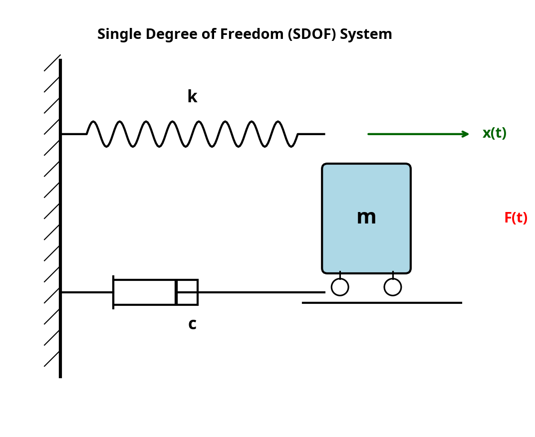Figure 1: Mass-spring-damper system showing the three fundamental elements

2. Derivation of the Equation of Motion

The equation of motion is derived by applying Newton's Second Law to the free-body diagram of the mass.

Free-Body Diagram Analysis

Consider the mass displaced by amount x from its equilibrium position:

1. Inertia force: mẍ (acts opposite to acceleration)
2. Spring force: -kx (restoring force toward equilibrium)
3. Damping force: -cẋ (opposes velocity)
4. External force: F(t) (applied excitation)

Applying ΣF = ma:

$F(t) - kx - c\dot{x} = m\ddot{x}$

Rearranging to standard form:

$\boxed{m\ddot{x} + c\dot{x} + kx = F(t)}$

This is the fundamental equation of motion for an SDOF system.

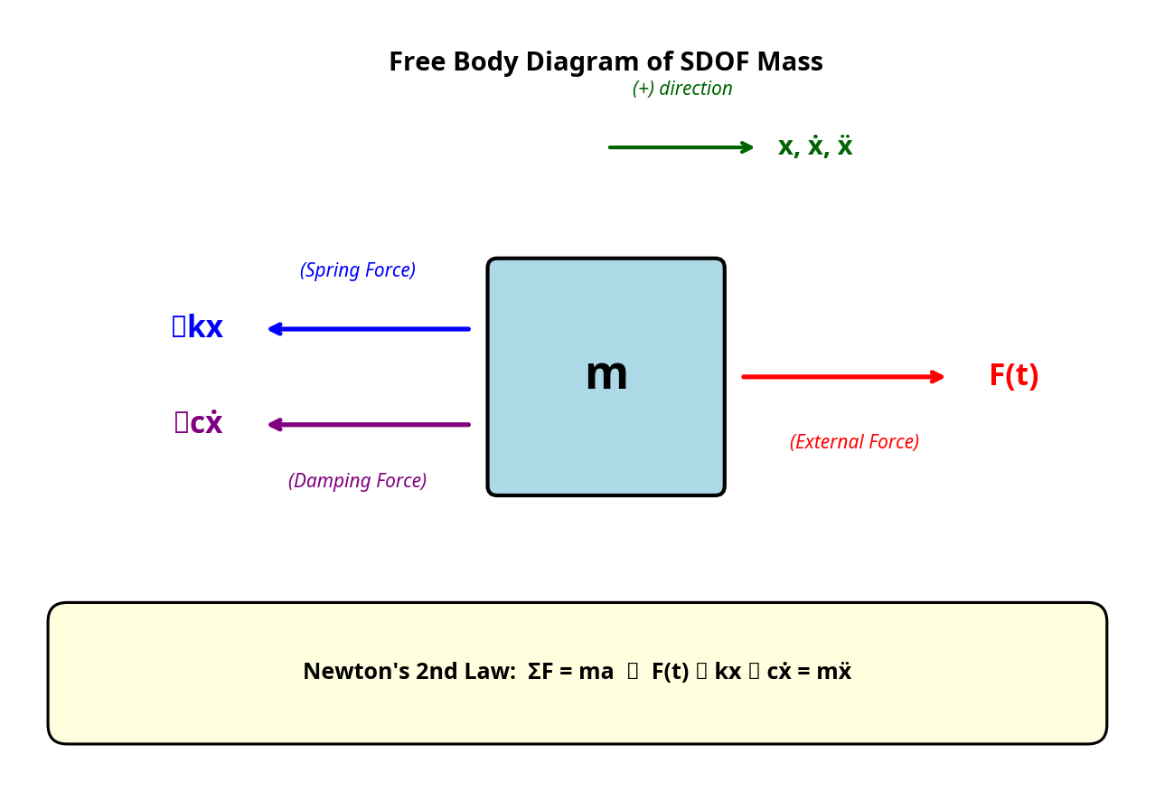
Figure 2: Free body diagram showing all forces acting on the mass. The spring force (-kx) and damping force (-cẋ) oppose the positive displacement and velocity directions respectively.

Normalized (Standard) Form

Dividing by mass m and introducing dimensionless parameters:

$\ddot{x} + 2\zeta\omega_n\dot{x} + \omega_n^2 x = \frac{F(t)}{m}$

Where:

• ωₙ = √(k/m) is the undamped natural frequency (rad/s)
• ζ = c/(2√km) = c/(2mωₙ) is the damping ratio (dimensionless)

3. Fundamental Parameters

Natural Frequency

The natural frequency represents how fast the system oscillates when disturbed and released:

$\omega_n = \sqrt{\frac{k}{m}} \quad \text{(rad/s)}$

$f_n = \frac{\omega_n}{2\pi} = \frac{1}{2\pi}\sqrt{\frac{k}{m}} \quad \text{(Hz)}$

Physical interpretation: A stiffer spring (higher k) increases frequency; more mass (higher m) decreases frequency. This is why a guitar string sounds higher when tightened (increased k) and lower when thicker (increased m).

Damping Ratio

The damping ratio ζ characterizes how quickly oscillations decay:

$\zeta = \frac{c}{c_{cr}} = \frac{c}{2\sqrt{km}} = \frac{c}{2m\omega_n}$

where c_cr = 2√(km) is the critical damping coefficient—the minimum damping required to prevent oscillation.

Typical values: Most mechanical structures have ζ = 0.01 to 0.05 (1-5%). Rubber mounts may reach ζ = 0.1-0.2. Critically damped systems (ζ = 1) are used in door closers and instrument needles.

Quality Factor (Q)

The quality factor is the inverse of twice the damping ratio:

$Q = \frac{1}{2\zeta}$

Physical interpretation: Q represents the amplification at resonance and the "sharpness" of the resonance peak. A high-Q system (low damping) has a narrow, tall resonance peak; a low-Q system has a broad, short peak.

Loss Factor (η)

The loss factor relates to energy dissipation per cycle:

$\eta = 2\zeta = \frac{1}{Q}$

This parameter is commonly used in structural damping and acoustic applications.

4. Types of Damping

Understanding different damping mechanisms is essential for accurate modeling. Each type has distinct physical origins and mathematical representations.

4.1 Viscous Damping

Physical mechanism: Energy dissipation through fluid resistance (dashpots, air resistance, oil dampers).

Force-velocity relationship: Linear and proportional to velocity

$F_d = c\dot{x}$

Energy dissipated per cycle (for harmonic motion x = X sin(ωt)):

$E_d = \pi c \omega X^2$

Energy dissipation is proportional to frequency—more energy is lost at higher frequencies.

Where it applies: Hydraulic dampers, shock absorbers, viscous fluid dampers.

4.2 Structural (Hysteretic) Damping

Physical mechanism: Internal friction within materials due to molecular-level slip and dislocation movement. Energy is lost through the stress-strain hysteresis loop.

Key characteristic: Energy dissipated per cycle is independent of frequency (unlike viscous damping).

$E_d = \pi \eta k X^2$

where η is the loss factor (material property).

Complex stiffness representation: Structural damping is elegantly represented using complex stiffness:

$k^* = k(1 + i\eta)$*

The equation of motion becomes:

$m\ddot{x} + k(1 + i\eta)x = F(t)$

Equivalent viscous damping: To use viscous damping equations with structural damping, define an equivalent viscous damping coefficient:

$c_{eq} = \frac{\eta k}{\omega}$

This equivalence is valid only at a specific frequency ω.

Where it applies: Metals, composites, bolted joints, welded structures.

4.3 Coulomb (Dry Friction) Damping

Physical mechanism: Sliding friction between dry surfaces. The friction force has constant magnitude but opposes the direction of motion.

$F_d = \mu N \cdot \text{sgn}(\dot{x})$

where μ is the coefficient of friction and N is the normal force.

Characteristics:

• Force magnitude is constant, independent of velocity
• Causes linear decay of amplitude (not exponential like viscous)
• Motion stops when restoring force < friction force (dead zone)
• Energy dissipated per cycle: E_d = 4μNX

Where it applies: Sliding joints, brake systems, friction dampers.

4.4 Comparison of Damping Types

Structural damping is linear in the frequency domain using complex stiffness.

4.5 Equivalent Viscous Damping

For analysis convenience, any damping mechanism can be converted to an equivalent viscous damping coefficient by equating energy dissipated per cycle:

$c_{eq} = \frac{E_d}{\pi \omega X^2}$

For structural damping: $c_{eq} = \frac{\eta k}{\omega} \quad \Rightarrow \quad \zeta_{eq} = \frac{\eta}{2} \cdot \frac{\omega_n}{\omega}$

At resonance (ω = ωₙ): ζ_eq = η/2, confirming that η = 2ζ.

For Coulomb damping: $c_{eq} = \frac{4\mu N}{\pi \omega X}$

Note: Coulomb equivalent damping depends on amplitude X, making it amplitude-dependent.

5. Free Vibration Response

Free vibration occurs when the system is disturbed from equilibrium and released with no external forcing (F(t) = 0).

General Solution

The homogeneous equation: $m\ddot{x} + c\dot{x} + kx = 0$

Assuming solution x = Ae^(st), the characteristic equation is: $ms^2 + cs + k = 0$

$s_{1,2} = -\zeta\omega_n \pm \omega_n\sqrt{\zeta^2 - 1}$

Underdamped Response (0 < ζ < 1)

For most engineering structures:

$x(t) = Xe^{-\zeta\omega_n t}\cos(\omega_d t - \phi)$

where:

• ωd = ωₙ√(1-ζ²) is the damped natural frequency
• X and φ are determined by initial conditions

Key insight: The damped frequency ωd is always less than the undamped frequency ωₙ. For typical damping (ζ < 0.1), the difference is negligible: ωd ≈ 0.995ωₙ at ζ = 0.1.

Logarithmic Decrement

The logarithmic decrement δ measures the rate of amplitude decay:

$\delta = \ln\left(\frac{x_n}{x_{n+1}}\right) = \frac{2\pi\zeta}{\sqrt{1-\zeta^2}}$

Practical approximation (for ζ < 0.1): $\delta \approx 2\pi\zeta \quad \Rightarrow \quad \zeta \approx \frac{\delta}{2\pi}$

Measuring damping from test data: Count n cycles and measure amplitude ratio: $\delta = \frac{1}{n}\ln\left(\frac{x_0}{x_n}\right)$

6. Forced Vibration Response

Harmonic Excitation

For sinusoidal forcing F(t) = F₀ sin(ωt), the steady-state response is:

$x(t) = X\sin(\omega t - \phi)$

where the amplitude X and phase φ depend on the frequency ratio r = ω/ωₙ.

Frequency Response Function (FRF)

The complex frequency response function H(ω) relates output to input:

$H(\omega) = \frac{X}{F_0/k} = \frac{1}{(1-r^2) + i(2\zeta r)}$

Magnitude (Dynamic Magnification Factor): $|H(\omega)| = DMF = \frac{1}{\sqrt{(1-r^2)^2 + (2\zeta r)^2}}$

Phase angle: $\phi = \tan^{-1}\left(\frac{2\zeta r}{1-r^2}\right)$

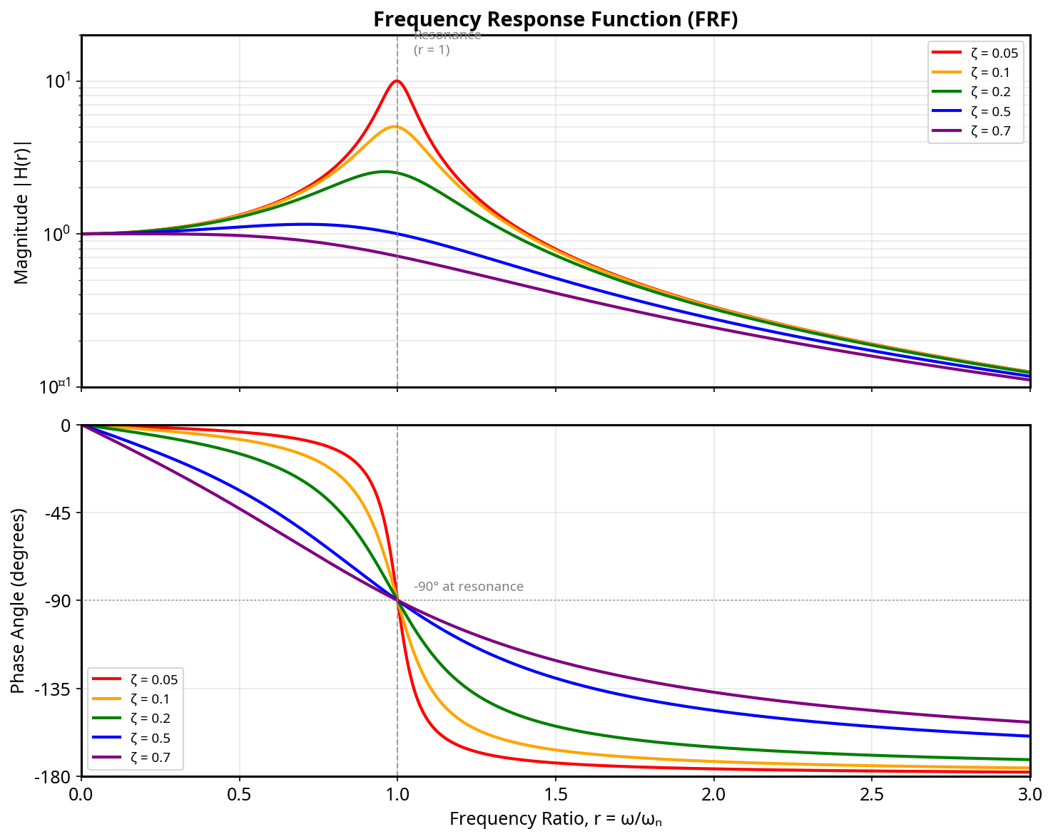
Figure: Magnitude and phase of the frequency response function (FRF). At resonance (r=1), the phase is -90° and magnitude is controlled by damping.

Key Frequency Response Characteristics

At resonance (r = 1): $DMF_{max} = Q = \frac{1}{2\zeta}$

The response amplitude is Q times the static deflection. For ζ = 0.02, this means 25× amplification!

Half-Power Bandwidth Method

The half-power bandwidth provides a practical method to measure damping from frequency response data.

Definition: The half-power points occur where the response power is half the peak value, corresponding to amplitude = peak/√2.

The frequencies at half-power points are: $r_1 \approx 1 - \zeta, \quad r_2 \approx 1 + \zeta$

Damping from bandwidth: $\zeta = \frac{f_2 - f_1}{2f_n} = \frac{\Delta f}{2f_n}$

Or equivalently: $Q = \frac{f_n}{\Delta f}$

This method is widely used in modal testing to extract damping from measured FRFs.

7. Base Excitation and Transmissibility

Many practical problems involve base motion rather than direct force application (e.g., earthquake excitation, vehicle suspension).

Problem Setup

The base moves with displacement y(t), and we want to find the mass response x(t).

Equation of motion (in terms of relative displacement z = x - y): $m\ddot{z} + c\dot{z} + kz = -m\ddot{y}$

Displacement Transmissibility

For harmonic base motion y = Y sin(ωt):

$T_d = \frac{X}{Y} = \sqrt{\frac{1 + (2\zeta r)^2}{(1-r^2)^2 + (2\zeta r)^2}}$

Force Transmissibility

The force transmitted to the base through the spring and damper:

$T_f = \frac{F_{transmitted}}{kY} = r^2 \cdot T_d$

Key Transmissibility Observations

Critical insight: Isolation only begins above r = √2 (regardless of damping). Below this frequency, the system amplifies base motion.

Damping trade-off: At resonance, more damping reduces amplification (good). In the isolation region, more damping reduces isolation effectiveness (bad). This trade-off is fundamental to isolator design.

8. Impulse Response and Convolution

Unit Impulse Response

The response to a unit impulse (Dirac delta function) is:

$h(t) = \frac{1}{m\omega_d}e^{-\zeta\omega_n t}\sin(\omega_d t), \quad t \geq 0$

This is the system's "signature"—it completely characterizes the dynamic behavior.

Convolution Integral (Duhamel's Integral)

For arbitrary forcing F(t), the response is:

$x(t) = \int_0^t F(\tau) h(t-\tau) d\tau$

$x(t) = \frac{1}{m\omega_d}\int_0^t F(\tau) e^{-\zeta\omega_n(t-\tau)}\sin[\omega_d(t-\tau)] d\tau$

Physical interpretation: The response at time t is the superposition of responses to all previous impulses F(τ)dτ, each weighted by the impulse response function.

Response to Common Inputs

9. Energy Methods

Energy methods provide physical insight and alternative solution approaches.

Kinetic Energy

$T = \frac{1}{2}m\dot{x}^2$

Maximum when passing through equilibrium (maximum velocity).

Potential Energy

$U = \frac{1}{2}kx^2$

Maximum at extreme displacement (zero velocity).

Energy Conservation (Undamped)

For undamped free vibration, total mechanical energy is constant:

$E = T + U = \frac{1}{2}m\dot{x}^2 + \frac{1}{2}kx^2 = \text{constant}$

This leads to an alternative derivation of natural frequency by equating maximum kinetic and potential energies:

$\frac{1}{2}m(\omega_n X)^2 = \frac{1}{2}kX^2 \quad \Rightarrow \quad \omega_n = \sqrt{\frac{k}{m}}$

Power Dissipation

For viscous damping, instantaneous power dissipated:

$P_d = c\dot{x}^2$

Average power over one cycle (harmonic motion):

$\bar{P}_d = \frac{1}{2}c\omega^2 X^2$

Energy Dissipated Per Cycle

$E_d = \oint F_d \, dx = \pi c \omega X^2$

This forms the basis for equivalent viscous damping calculations.

10. Miles' Equation: Complete Derivation

Miles' equation estimates the RMS response of an SDOF system to random vibration with a flat (white noise) PSD input. This is fundamental to random vibration analysis.

Problem Statement

Given:

• SDOF system with natural frequency fₙ and quality factor Q
• Base acceleration PSD: W₀ (g²/Hz), assumed constant (white noise)

Find: RMS acceleration response of the mass

Derivation

Step 1: Response PSD

The output PSD is related to input PSD through the squared magnitude of the FRF:

$S_{out}(f) = |H(f)|^2 \cdot S_{in}(f)$

For acceleration response to base acceleration:

$S_{\ddot{x}}(f) = |H(f)|^2 \cdot W_0$

where: $|H(f)|^2 = \frac{1 + (2\zeta r)^2}{(1-r^2)^2 + (2\zeta r)^2}$

Step 2: Mean Square Response

The mean square response is the integral of the response PSD:

$\ddot{x}_{rms}^2 = \int_0^\infty S_{\ddot{x}}(f) \, df = W_0 \int_0^\infty |H(f)|^2 \, df$

Step 3: Evaluate the Integral

The key integral is: $I = \int_0^\infty \frac{1 + (2\zeta r)^2}{(1-r^2)^2 + (2\zeta r)^2} \, df$

Substituting r = f/fₙ and df = fₙ dr:

$I = f_n \int_0^\infty \frac{1 + (2\zeta r)^2}{(1-r^2)^2 + (2\zeta r)^2} \, dr$

This integral has a closed-form solution (derived using residue theory):

$\int_0^\infty \frac{1 + (2\zeta r)^2}{(1-r^2)^2 + (2\zeta r)^2} \, dr = \frac{\pi}{4\zeta}(1 + 4\zeta^2)$

Step 4: Simplify for Light Damping

For typical structures (ζ << 1), the term 4ζ² << 1, so:

$I \approx f_n \cdot \frac{\pi}{4\zeta} = \frac{\pi f_n Q}{2}$

Step 5: Final Result

$\ddot{x}_{rms}^2 = W_0 \cdot \frac{\pi f_n Q}{2}$

$\boxed{\ddot{x}_{rms} = \sqrt{\frac{\pi}{2} f_n Q \cdot W_0}}$

Key Assumptions

1. White noise input: PSD is constant across all frequencies
2. Light damping: ζ << 1 (Q >> 1)
3. Linear system: Superposition applies
4. Stationary random process: Statistics don't change with time

Practical Form

Often written as:

$G_{rms} = \sqrt{\frac{\pi}{2} f_n Q \cdot W_0} \quad \text{(in g's if } W_0 \text{ is in g}^2\text{/Hz)}$

Worked Example

Given: Component with fₙ = 100 Hz, Q = 25, subjected to W₀ = 0.04 g²/Hz

Solution: $G_{rms} = \sqrt{\frac{\pi}{2} \times 100 \times 25 \times 0.04} = \sqrt{157.1} = 12.5 \text{ g}$

3σ peak: Assuming Gaussian distribution, 99.7% of peaks are within 3σ: $G_{3\sigma} = 3 \times 12.5 = 37.5 \text{ g}$

11. Response Spectrum Concepts

The response spectrum connects SDOF dynamics to shock and transient analysis.

Shock Response Spectrum (SRS)

The SRS plots the maximum response of SDOF oscillators (with varying natural frequencies) to a given transient input.

Definition: For each natural frequency fₙ: $SRS(f_n) = \max_t |x(t)| \cdot \omega_n^2 \quad \text{(for acceleration)}$

Physical interpretation: The SRS answers: "What is the worst-case response a component with natural frequency fₙ will experience from this shock?"

Types of SRS

SRS and Damage Potential

Two shocks with identical SRS will produce the same maximum response in any SDOF system, making SRS a measure of damage potential regardless of the specific time history.

12. Practical Applications and Common Pitfalls

Isolator Design Example

Problem: Design an isolator to achieve 80% isolation (T = 0.2) at 50 Hz.

Solution: From T = 0.2 and assuming light damping in isolation region: $T \approx \frac{1}{r^2 - 1} = 0.2$ $r^2 = 6 \quad \Rightarrow \quad r = 2.45$

Required natural frequency: $f_n = \frac{50}{2.45} = 20.4 \text{ Hz}$

Required stiffness (for 10 kg mass): $k = m(2\pi f_n)^2 = 10 \times (2\pi \times 20.4)^2 = 164,000 \text{ N/m}$

Common Pitfalls

1. Confusing ω and f: Always check units. ω is in rad/s, f is in Hz. They differ by factor of 2π.

2. Forgetting the √2 crossover: Isolation only occurs above r = √2 ≈ 1.41. Designing an isolator with fₙ close to the excitation frequency will amplify, not isolate.

3. Ignoring damping trade-offs: More damping helps at resonance but hurts isolation. Optimal damping depends on the operating frequency range.

4. Assuming Q = 1/(2ζ) always applies: This relationship assumes viscous damping. For structural damping, Q = 1/η.

5. Using Miles' equation outside its assumptions: Miles' equation assumes white noise input. For shaped spectra, numerical integration is required.

13. Check Your Learning

Test your understanding with these fundamental questions:

Conceptual Questions

1. Why does increasing mass decrease natural frequency while increasing stiffness increases it?

2. Explain physically why the phase angle is 90° at resonance.

3. Why does isolation only begin above r = √2, regardless of damping level?

4. What is the physical difference between viscous and structural damping? How does energy dissipation differ with frequency?

5. Why is the damped natural frequency always less than the undamped natural frequency?

6. Explain why more damping is beneficial at resonance but detrimental in the isolation region.

7. What assumptions are required for Miles' equation to be valid?

8. How would you measure damping ratio from a free vibration decay test?

9. What does the quality factor Q physically represent?

10. Why is the SRS a useful metric for comparing shock severity?

Derivation Exercises

1. Starting from Newton's Second Law, derive the equation of motion for an SDOF system.

2. Derive the expression for logarithmic decrement in terms of damping ratio.

3. Show that the half-power bandwidth method gives ζ = Δf/(2fₙ).

4. Derive the transmissibility equation for base excitation.

5. Starting from the FRF, derive Miles' equation for RMS response.

Numerical Problems

1. A system has m = 5 kg, k = 20,000 N/m, c = 50 N·s/m. Calculate fₙ, ζ, Q, and ωd.

2. An oscillator decays from 10 mm to 2 mm amplitude in 8 cycles. What is the damping ratio?

3. Design an isolator to achieve 90% isolation at 100 Hz for a 2 kg mass. What stiffness is required?

4. A component (fₙ = 200 Hz, Q = 20) is exposed to 0.1 g²/Hz random vibration. What is the 3σ acceleration?

14. Key Equations to Memorize

Fundamental Parameters

Response Equations

Quick Reference Values

Damping Relationships

---

Try It Yourself

Explore these concepts interactively:

• SDOF Response Calculator — Visualize time and frequency response
• G-RMS Calculator — Apply Miles' equation to real PSD data
• SRS Calculator — Generate shock response spectra

---

This tutorial is part of the VS&A All Day Engineering Education series.

References

[1] Rao, S. S. (2017). Mechanical Vibrations (6th ed.). Pearson.

[2] Thomson, W. T., & Dahleh, M. D. (1998). Theory of Vibration with Applications (5th ed.). Prentice Hall.

[3] Inman, D. J. (2014). Engineering Vibration (4th ed.). Pearson.

[4] Harris, C. M., & Piersol, A. G. (2002). Harris' Shock and Vibration Handbook (5th ed.). McGraw-Hill.

[5] Irvine, T. (2023). "Miles Equation." Vibrationdata.com.

---

14. Multi-Degree of Freedom (MDOF) Systems

Understanding MDOF systems is the natural extension of SDOF analysis. Real structures have infinite degrees of freedom, but we approximate them with finite DOF models. The key insight is that any MDOF system can be decomposed into a set of independent SDOF systems through modal analysis—this is why mastering SDOF fundamentals is so critical.

14.1 The Matrix Equation of Motion

For an N-DOF system, the equation of motion becomes a matrix equation:

$\mathbf{[M]\{\ddot{x}\} + [C]\{\dot{x}\} + [K]\{x\} = \{F(t)\}}$

Where:

• [M] is the N×N mass matrix (symmetric, positive definite)
• [C] is the N×N damping matrix (symmetric)
• [K] is the N×N stiffness matrix (symmetric, positive semi-definite)
• {x} is the N×1 displacement vector
• {F(t)} is the N×1 force vector

14.2 Derivation: 2-DOF System Example

Consider two masses connected by springs:

Free-body diagram for m₁:

• Spring 1 force: -k₁x₁ (pulls back toward wall)
• Spring 2 force: -k₂(x₁ - x₂) (interaction with m₂)

Applying Newton's Second Law to m₁: $m_1\ddot{x}_1 = -k_1x_1 - k_2(x_1 - x_2)$ $m_1\ddot{x}_1 + (k_1 + k_2)x_1 - k_2x_2 = 0$

Free-body diagram for m₂:

• Spring 2 force: -k₂(x₂ - x₁)
• Spring 3 force: -k₃x₂

Applying Newton's Second Law to m₂: $m_2\ddot{x}_2 = -k_2(x_2 - x_1) - k_3x_2$ $m_2\ddot{x}_2 - k_2x_1 + (k_2 + k_3)x_2 = 0$

Matrix form:

$\begin{bmatrix} m_1 & 0 \\ 0 & m_2 \end{bmatrix} \begin{Bmatrix} \ddot{x}_1 \\ \ddot{x}_2 \end{Bmatrix} + \begin{bmatrix} k_1+k_2 & -k_2 \\ -k_2 & k_2+k_3 \end{bmatrix} \begin{Bmatrix} x_1 \\ x_2 \end{Bmatrix} = \begin{Bmatrix} 0 \\ 0 \end{Bmatrix}$

Key observations:

• Mass matrix is diagonal (lumped mass model)
• Stiffness matrix is symmetric (Maxwell's reciprocity)
• Off-diagonal terms represent coupling between DOFs

14.3 The Eigenvalue Problem

To find natural frequencies and mode shapes, assume harmonic motion:

$\{x\} = \{\phi\}e^{i\omega t}$

Substituting into the undamped equation of motion:

$-\omega^2[M]\{\phi\} + [K]\{\phi\} = \{0\}$

Rearranging:

$\boxed{[K]\{\phi\} = \omega^2[M]\{\phi\}}$

This is the generalized eigenvalue problem. The solutions are:

• Eigenvalues λᵢ = ωᵢ² (squared natural frequencies)
• Eigenvectors {φ}ᵢ (mode shapes)

Standard form (pre-multiply by [M]⁻¹): $[M]^{-1}[K]\{\phi\} = \omega^2\{\phi\}$

or equivalently: $[A]\{\phi\} = \lambda\{\phi\}$

where [A] = [M]⁻¹[K] is the dynamic matrix and λ = ω².

14.4 Solving the Eigenvalue Problem

Characteristic equation: $\det([K] - \omega^2[M]) = 0$

This yields an Nth-order polynomial in ω², giving N natural frequencies.

2-DOF Example (Numerical):

Let m₁ = m₂ = 1 kg, k₁ = k₃ = 1 N/m, k₂ = 2 N/m:

$[M] = \begin{bmatrix} 1 & 0 \\ 0 & 1 \end{bmatrix}, \quad [K] = \begin{bmatrix} 3 & -2 \\ -2 & 3 \end{bmatrix}$

Characteristic equation: $\det\begin{bmatrix} 3-\omega^2 & -2 \\ -2 & 3-\omega^2 \end{bmatrix} = 0$

$(3-\omega^2)^2 - 4 = 0$ $9 - 6\omega^2 + \omega^4 - 4 = 0$ $\omega^4 - 6\omega^2 + 5 = 0$

Using quadratic formula with u = ω²: $u = \frac{6 \pm \sqrt{36-20}}{2} = \frac{6 \pm 4}{2}$

Natural frequencies:

• ω₁² = 1 → ω₁ = 1 rad/s (f₁ = 0.159 Hz)
• ω₂² = 5 → ω₂ = 2.236 rad/s (f₂ = 0.356 Hz)

14.5 Mode Shapes and Physical Interpretation

Finding mode shapes:

For ω₁² = 1, substitute into eigenvalue equation: $\begin{bmatrix} 3-1 & -2 \\ -2 & 3-1 \end{bmatrix} \begin{Bmatrix} \phi_{11} \\ \phi_{21} \end{Bmatrix} = \begin{Bmatrix} 0 \\ 0 \end{Bmatrix}$

$2\phi_{11} - 2\phi_{21} = 0 \Rightarrow \phi_{11} = \phi_{21}$

Mode 1: {φ}₁ = {1, 1}ᵀ (in-phase motion, both masses move together)

For ω₂² = 5: $\begin{bmatrix} 3-5 & -2 \\ -2 & 3-5 \end{bmatrix} \begin{Bmatrix} \phi_{12} \\ \phi_{22} \end{Bmatrix} = \begin{Bmatrix} 0 \\ 0 \end{Bmatrix}$

$-2\phi_{12} - 2\phi_{22} = 0 \Rightarrow \phi_{12} = -\phi_{22}$

Mode 2: {φ}₂ = {1, -1}ᵀ (out-of-phase motion, masses move opposite)

Physical interpretation:

• Mode 1 (lower frequency): Masses move in the same direction—the middle spring (k₂) doesn't stretch, so effective stiffness is lower
• Mode 2 (higher frequency): Masses move in opposite directions—the middle spring stretches twice as much, so effective stiffness is higher

14.6 Orthogonality of Mode Shapes

Mode shapes possess a crucial mathematical property—orthogonality with respect to mass and stiffness matrices:

$\{\phi\}_i^T[M]\{\phi\}_j = 0 \quad \text{for } i \neq j$ $\{\phi\}_i^T[K]\{\phi\}_j = 0 \quad \text{for } i \neq j$

Why this matters: Orthogonality allows us to decouple the N coupled equations into N independent SDOF equations.

Modal mass and stiffness: $M_i = \{\phi\}_i^T[M]\{\phi\}_i \quad \text{(generalized mass)}$ $K_i = \{\phi\}_i^T[K]\{\phi\}_i \quad \text{(generalized stiffness)}$

Verification: ωᵢ² = Kᵢ/Mᵢ

14.7 Modal Superposition Method

The total response is a linear combination of modal responses:

$\{x(t)\} = \sum_{i=1}^{N} \{\phi\}_i q_i(t) = [\Phi]\{q(t)\}$

Where:

• [\Phi] is the modal matrix (columns are mode shapes)
• {q(t)} is the vector of modal coordinates (generalized coordinates)

Decoupled equations:

Substituting into the equation of motion and pre-multiplying by {φ}ᵢᵀ:

$M_i\ddot{q}_i + C_i\dot{q}_i + K_i q_i = F_i(t)$

This is an SDOF equation for each mode! The modal force is: $F_i(t) = \{\phi\}_i^T\{F(t)\}$

Solution procedure:

1. Solve eigenvalue problem → ωᵢ, {φ}ᵢ
2. Calculate modal parameters: Mᵢ, Kᵢ, Cᵢ, Fᵢ(t)
3. Solve N independent SDOF problems for qᵢ(t)
4. Reconstruct physical response: {x(t)} = Σ{φ}ᵢqᵢ(t)

14.8 Modal Participation and Effective Mass

Not all modes contribute equally to the response. The modal participation factor quantifies each mode's contribution:

$\Gamma_i = \frac{\{\phi\}_i^T[M]\{r\}}{M_i}$

Where {r} is the influence vector (direction of excitation).

Effective modal mass: $M_{eff,i} = \frac{(\{\phi\}_i^T[M]\{r\})^2}{M_i}$

Key insight: The sum of effective masses equals the total mass: $\sum_{i=1}^{N} M_{eff,i} = \{r\}^T[M]\{r\}$

This is used to determine how many modes to include in analysis (typically until 90% of mass is captured).

14.9 Proportional (Rayleigh) Damping

For MDOF systems, damping is often assumed proportional to mass and stiffness:

$[C] = \alpha[M] + \beta[K]$

Why use this? Proportional damping preserves mode shapes and allows modal decoupling.

Determining α and β:

Given damping ratios ζᵢ and ζⱼ at two frequencies:

$\zeta_i = \frac{\alpha}{2\omega_i} + \frac{\beta\omega_i}{2}$ $\zeta_j = \frac{\alpha}{2\omega_j} + \frac{\beta\omega_j}{2}$

Solving simultaneously: $\alpha = \frac{2\omega_i\omega_j(\zeta_i\omega_j - \zeta_j\omega_i)}{\omega_j^2 - \omega_i^2}$ $\beta = \frac{2(\zeta_j\omega_j - \zeta_i\omega_i)}{\omega_j^2 - \omega_i^2}$

Common simplification: If ζᵢ = ζⱼ = ζ: $\alpha = \frac{2\zeta\omega_i\omega_j}{\omega_i + \omega_j}, \quad \beta = \frac{2\zeta}{\omega_i + \omega_j}$

14.10 Practical Considerations

Mode truncation: In practice, only the first several modes significantly affect response. Higher modes have:

• Higher frequencies (often above excitation bandwidth)
• Lower participation factors
• More damping (if using Rayleigh damping with β > 0)

Rigid body modes: Unconstrained structures have zero-frequency modes (rigid body translation/rotation). These have ω = 0 and represent motion without elastic deformation.

Repeated frequencies: Some symmetric structures have multiple modes at the same frequency (degenerate modes). Any linear combination of these modes is also a valid mode shape.

14.11 MDOF Response to Harmonic Excitation

For harmonic forcing {F(t)} = {F₀}e^(iωt), the steady-state response is:

$\{X\} = [H(\omega)]\{F_0\}$

Where [H(ω)] is the receptance matrix (frequency response function matrix):

$[H(\omega)] = \sum_{i=1}^{N} \frac{\{\phi\}_i\{\phi\}_i^T}{K_i - \omega^2 M_i + i\omega C_i}$

Each element Hⱼₖ(ω) represents the response at DOF j due to unit force at DOF k.

14.12 Connection to Finite Element Analysis

Modern structural dynamics uses FEA to generate [M] and [K] matrices:

1. Mesh the structure into elements
2. Assemble global matrices from element contributions
3. Apply boundary conditions (reduce matrix size)
4. Solve eigenvalue problem for modes
5. Perform modal superposition for dynamic response

The same SDOF and MDOF principles apply whether you have 2 DOFs or 2 million DOFs.

---

15. MDOF Check Your Learning

Test your understanding of multi-degree of freedom systems:

Conceptual Questions

1. Why is the stiffness matrix symmetric? What physical principle guarantees this?

2. If a 3-DOF system has natural frequencies of 10, 25, and 50 Hz, what are the eigenvalues of [M]⁻¹[K]?

3. A 2-DOF system has mode shapes {1, 0.5}ᵀ and {1, -2}ᵀ. Which mode has the higher natural frequency and why?

4. What does it mean physically when two modes are orthogonal with respect to the mass matrix?

5. Why does modal superposition work? What property of the mode shapes enables decoupling?

Calculation Questions

6. Given [M] = diag(2, 1) kg and [K] = [6, -2; -2, 2] N/m, find the natural frequencies.

7. For the system in Q6, find the mode shapes and verify orthogonality.

8. A structure has 100 DOFs. After modal analysis, the first 5 modes capture 92% of the effective mass. How many modes should you include in a dynamic analysis?

9. Using Rayleigh damping with ζ = 5% at 10 Hz and 100 Hz, what is the damping ratio at 50 Hz?

10. A 2-DOF system is excited at its first natural frequency. Which mode dominates the response?

Design Questions

11. You need to shift the first natural frequency of a 2-DOF system higher without changing the total mass. What design changes would you consider?

12. A vibration isolator is modeled as a 2-DOF system (equipment + intermediate mass). What are the advantages over a single-stage (SDOF) isolator?

---

16. MDOF Key Equations to Memorize

Matrix Equation of Motion

$[M]\{\ddot{x}\} + [C]\{\dot{x}\} + [K]\{x\} = \{F(t)\}$

Eigenvalue Problem

$[K]\{\phi\} = \omega^2[M]\{\phi\}$ $\det([K] - \omega^2[M]) = 0$

Orthogonality Conditions

$\{\phi\}_i^T[M]\{\phi\}_j = 0 \quad (i \neq j)$ $\{\phi\}_i^T[K]\{\phi\}_j = 0 \quad (i \neq j)$

Modal Parameters

$M_i = \{\phi\}_i^T[M]\{\phi\}_i$ $K_i = \{\phi\}_i^T[K]\{\phi\}_i$ $\omega_i^2 = K_i/M_i$

Modal Superposition

$\{x(t)\} = \sum_{i=1}^{N} \{\phi\}_i q_i(t)$ $M_i\ddot{q}_i + C_i\dot{q}_i + K_i q_i = \{\phi\}_i^T\{F(t)\}$

Modal Participation Factor

$\Gamma_i = \frac{\{\phi\}_i^T[M]\{r\}}{M_i}$

Effective Modal Mass

$M_{eff,i} = \frac{(\{\phi\}_i^T[M]\{r\})^2}{M_i}$

Rayleigh Damping

$[C] = \alpha[M] + \beta[K]$ $\zeta_i = \frac{\alpha}{2\omega_i} + \frac{\beta\omega_i}{2}$

---

17. Complete Dynamics Reference Card

A printable summary of all key equations from this guide is available for download.

Download PDF Cheat Sheet

Quick Reference: SDOF Fundamentals

Quick Reference: Response Equations

Quick Reference: Damping Types

Quick Reference: MDOF Essentials

---

18. Continuous Systems: The Bridge to FEA

While SDOF and MDOF models use discrete masses and springs, real structures are continuous—they have mass and stiffness distributed throughout their volume. Understanding continuous systems provides the theoretical foundation for finite element analysis and explains why FEA works.

The key insight: Continuous systems have infinite degrees of freedom, but their response can still be expressed as a sum of modes—just like MDOF systems. Each mode has a natural frequency and mode shape, and the same orthogonality and superposition principles apply.

18.1 The Vibrating String

The string is the simplest continuous system and provides intuition for all others.

Governing equation (1D wave equation):

$\frac{\partial^2 y}{\partial t^2} = c^2 \frac{\partial^2 y}{\partial x^2}$

where c = √(T/ρA) is the wave speed, T is tension, ρ is density, and A is cross-sectional area.

Separation of variables: Assume y(x,t) = φ(x)q(t):

$\frac{1}{q}\frac{d^2q}{dt^2} = c^2 \frac{1}{\phi}\frac{d^2\phi}{dx^2} = -\omega^2$

This separates into two ODEs:

• Time equation: q̈ + ω²q = 0 (simple harmonic motion)
• Spatial equation: φ'' + (ω/c)²φ = 0 (mode shape equation)

Solution for fixed-fixed string (length L):

Mode shapes: $\phi_n(x) = \sin\left(\frac{n\pi x}{L}\right)$

Natural frequencies: $f_n = \frac{n}{2L}\sqrt{\frac{T}{\rho A}} = \frac{nc}{2L}$

Physical interpretation: The modes are standing waves. Mode 1 (n=1) is the fundamental with one half-wavelength fitting in L. Mode 2 has two half-wavelengths, etc. The frequencies are integer multiples of the fundamental—this is why strings produce harmonic overtones.

18.2 Longitudinal Vibration of Rods

A rod vibrating axially follows the same wave equation as a string:

$\frac{\partial^2 u}{\partial t^2} = c_L^2 \frac{\partial^2 u}{\partial x^2}$

where c_L = √(E/ρ) is the longitudinal wave speed, E is Young's modulus.

Fixed-free rod (cantilever):

Mode shapes: $\phi_n(x) = \sin\left(\frac{(2n-1)\pi x}{2L}\right)$

Natural frequencies: $f_n = \frac{(2n-1)}{4L}\sqrt{\frac{E}{\rho}}$

Key observation: Only odd harmonics exist for fixed-free boundary conditions. The fundamental has a quarter-wavelength in the rod length.

Fixed-fixed rod:

Natural frequencies: $f_n = \frac{n}{2L}\sqrt{\frac{E}{\rho}}$

Same as the string—integer multiples of the fundamental.

18.3 Transverse Vibration of Beams

Beam bending is more complex because it involves fourth-order spatial derivatives.

Euler-Bernoulli beam equation:

$EI\frac{\partial^4 y}{\partial x^4} + \rho A\frac{\partial^2 y}{\partial t^2} = 0$

where EI is the flexural rigidity and ρA is mass per unit length.

Characteristic equation: Assuming y(x,t) = φ(x)e^(iωt):

$\frac{d^4\phi}{dx^4} = \beta^4\phi$

where $\beta^4 = \frac{\rho A \omega^2}{EI}$

General solution:

$\phi(x) = C_1\cosh(\beta x) + C_2\sinh(\beta x) + C_3\cos(\beta x) + C_4\sin(\beta x)$

The four constants are determined by four boundary conditions (two at each end).

18.4 Beam Boundary Conditions

18.5 Beam Natural Frequencies

The natural frequency formula for any beam is:

$f_n = \frac{(\beta_n L)^2}{2\pi L^2}\sqrt{\frac{EI}{\rho A}}$

where (βₙL) depends on boundary conditions:

Key observations:

• Simply supported beam has frequencies proportional to n² (like a string squared)
• Cantilever has the lowest fundamental frequency for a given length
• Fixed-fixed and free-free have identical frequencies (reciprocity)
• Higher modes are NOT integer multiples of the fundamental (unlike strings)

18.6 Worked Example: Cantilever Beam

Problem: Find the first three natural frequencies of an aluminum cantilever beam.

• Length L = 0.5 m
• Width b = 25 mm, Height h = 5 mm (rectangular cross-section)
• E = 70 GPa, ρ = 2700 kg/m³

Step 1: Calculate section properties

$I = \frac{bh^3}{12} = \frac{(0.025)(0.005)^3}{12} = 2.604 \times 10^{-10} \text{ m}^4$

$A = bh = (0.025)(0.005) = 1.25 \times 10^{-4} \text{ m}^2$

Step 2: Calculate the frequency coefficient

$\frac{1}{2\pi L^2}\sqrt{\frac{EI}{\rho A}} = \frac{1}{2\pi (0.5)^2}\sqrt{\frac{(70 \times 10^9)(2.604 \times 10^{-10})}{(2700)(1.25 \times 10^{-4})}}$

$= \frac{1}{1.571}\sqrt{\frac{18.23}{0.3375}} = 0.637 \times 7.35 = 4.68 \text{ Hz}$

Step 3: Apply (βₙL)² values for cantilever

Verification: The frequency ratios are 1 : 6.24 : 17.5, matching the theoretical cantilever ratios.

18.7 Cantilever Mode Shapes

The mode shapes for a cantilever beam are:

$\phi_n(x) = \cosh(\beta_n x) - \cos(\beta_n x) - \sigma_n[\sinh(\beta_n x) - \sin(\beta_n x)]$

where $\sigma_n = \frac{\cosh(\beta_n L) + \cos(\beta_n L)}{\sinh(\beta_n L) + \sin(\beta_n L)}$

Physical interpretation:

• Mode 1: The entire beam bends in one direction
• Mode 2: One internal node where displacement is zero
• Mode 3: Two internal nodes
• Each higher mode adds one more node

18.8 Plate Vibration

Plates extend beam theory to two dimensions.

Governing equation (thin plate):

$D\nabla^4 w + \rho h\frac{\partial^2 w}{\partial t^2} = 0$

where D = Eh³/[12(1-ν²)] is the flexural rigidity, h is thickness, and ∇⁴ is the biharmonic operator.

Simply supported rectangular plate (a × b):

Mode shapes: $\phi_{mn}(x,y) = \sin\left(\frac{m\pi x}{a}\right)\sin\left(\frac{n\pi y}{b}\right)$

Natural frequencies: $f_{mn} = \frac{\pi}{2}\sqrt{\frac{D}{\rho h}}\left[\left(\frac{m}{a}\right)^2 + \left(\frac{n}{b}\right)^2\right]$

Key observations:

• Plates have two mode indices (m, n) for the two spatial directions
• Mode (1,1) is the fundamental—one half-wave in each direction
• Modes can be degenerate (same frequency) for square plates when m and n are swapped
• Plate modes are more complex than beam modes due to 2D nature

18.9 Connection to Finite Element Analysis

FEA discretizes continuous systems into MDOF systems. Understanding this connection is crucial:

How FEA approximates continuous systems:

1. Mesh the structure into elements (beams, shells, solids)
2. Assume displacement interpolation within each element using shape functions
3. Assemble element matrices into global [M] and [K]
4. Solve the eigenvalue problem [K]{φ} = ω²[M]{φ}

Why it works: The FEA mode shapes are approximations to the true continuous mode shapes. As the mesh is refined:

• More DOFs → better approximation of higher modes
• Lower modes converge faster than higher modes
• The FEA frequencies approach the analytical values from above (Rayleigh's theorem)

Mesh density rule of thumb:

• Need 6-10 linear elements per wavelength
• Need 3-4 quadratic elements per wavelength
• For bending: λ_bending = 2π/β, where β⁴ = ρAω²/(EI)

Example: To capture modes up to 1000 Hz in a steel beam (E = 200 GPa, ρ = 7800 kg/m³, h = 10 mm):

$\lambda_{bending} = 2\pi\left(\frac{EI}{\rho A \omega^2}\right)^{1/4} \approx 0.12 \text{ m at 1000 Hz}$

Element size ≤ λ/6 ≈ 20 mm for linear elements.

18.10 Modal Density and Statistical Energy Analysis

At high frequencies, modes become densely packed and individual mode identification becomes impractical. This leads to statistical approaches.

Modal density n(f) = number of modes per Hz:

Plate modal density (simply supported):

$n(f) = \frac{A}{2}\sqrt{\frac{12\rho(1-\nu^2)}{Eh^2}} = \frac{A\sqrt{3}}{h c_L}$

Key insight: Plate modal density is independent of frequency! This is why plates are efficient radiators and why Statistical Energy Analysis (SEA) works well for plate-dominated structures.

18.11 Continuous Systems Summary

The unifying theme: All continuous systems can be analyzed using:

1. Separation of variables → spatial modes + time response
2. Boundary conditions → determine allowable mode shapes
3. Orthogonality → enables modal superposition
4. Same principles as MDOF, just with infinite modes

---

19. Continuous Systems Check Your Learning

Test your understanding of continuous systems:

Conceptual Questions

1. Why do beam frequencies scale with (βL)² while string frequencies scale with n? What's fundamentally different about the governing equations?

2. A cantilever beam and a free-free beam of the same dimensions have the same second natural frequency. Why?

3. Why does a simply supported plate have constant modal density while a beam's modal density increases with frequency?

4. When would you use Euler-Bernoulli beam theory vs. Timoshenko beam theory?

5. Why do FEA frequencies always converge from above (overestimate) as the mesh is refined?

Calculation Questions

6. A guitar string (L = 0.65 m, T = 70 N, ρA = 0.001 kg/m) is tuned to E2 (82.4 Hz). Verify this is the fundamental frequency.

7. A steel cantilever beam (L = 0.3 m, b = 20 mm, h = 3 mm, E = 200 GPa, ρ = 7800 kg/m³) is used as a vibration sensor. What is its fundamental frequency?

8. For the beam in Q7, what element size would you use in FEA to accurately capture modes up to 500 Hz?

9. A simply supported square plate (0.5 m × 0.5 m × 2 mm steel) has what fundamental frequency? What is its modal density?

10. Two beams have the same fundamental frequency. Beam A is simply supported, Beam B is cantilever. What is the ratio of their lengths (L_A/L_B)?

---

20. Complete Dynamics Reference

This guide has covered the full spectrum of structural dynamics, from single degree of freedom systems through multi-degree of freedom analysis to continuous systems. The progression follows how real engineering problems are approached:

1. SDOF provides fundamental intuition about resonance, damping, and dynamic response
2. MDOF introduces modal analysis and the eigenvalue problem
3. Continuous systems show the theoretical basis for FEA and high-frequency analysis

The unifying principles across all systems:

• Natural frequencies and mode shapes characterize dynamic behavior
• Orthogonality enables modal superposition
• Damping dissipates energy and limits resonant response
• The same equations (just in different forms) apply at every scale

Master these fundamentals, and you'll have the foundation to tackle any structural dynamics problem—from component vibration testing to full vehicle modal analysis to acoustic fatigue assessment.

Download the complete PDF Cheat Sheet for a printable reference of all key equations.